Do you really need backlinks? (R tutorial)

“Everyone knows that backlinks can boost rankings on Google!”

Are you really sure?

You’ve probably already noticed it, it’s not uncommon to see pages positioned without ANY backlink. In this tutorial, I propose a first approach to analyze your backlinks needs in the form of an exploratory SERP analysis.

Prerequisites

We will use the R language and the R Studio IDE to run our script.

You will also need a Majestic API key, which will be used to automate the recovery of netlinking data.

If this is the first tool you develop with R, have no fear, I will explain a simplified method here and we will build the tool step by step.

What will we do here ?

I will show you an easy way to create a netlinking “pre-audit” tool. The tool will perform 3 operations :

• Retrieve the Top 100 URLs that rank on a keyword using web scraping
• Automatically retrieve more than 140 netlinking variables (CF, TF, Root Domain, etc.) for each URL, using the Majestic API and the majestic R package
• Analyze correlations between URL’s position on Google and their Majestic data

Ready to analyze the SERP? Let’s GO!

1. Install the R packages

The following code will check in your library if you already have the packages or not, and install them only if you don’t have them (A piece of code to keep close!).

list.of.packages <- c("stringr", "httr","XML", "dplyr", "majesticR","Hmisc","corrplot","PerformanceAnalytics")

new.packages <- list.of.packages[!(list.of.packages %in% installed.packages()[,"Package"])]
if(length(new.packages)) install.packages(new.packages)

library(stringr)
library(httr)
library(XML)
library(dplyr)
library(majesticR)
library(Hmisc)
library(corrplot)
library(PerformanceAnalytics)

2. Get the Google Top 100 URLs for a specific keyword

We start by creating our SERP scraper that we will call get_google_serp_urls(). This is a function that will build the SERP URL from a keyword, retrieve the content, then extract the URLs.

The function takes 5 parameters:

• querie : the keyword you want to study the SERP
• number_of_results : the number of Google results you want to recover (10, 100, etc.)
• country_code : SERP country (see the country code list on Wikipedia)
• language_code : SERP language (see the list on Wikipédia)
• user_agent : the user agent with whom you want to make the request

Copy and paste the following code into an R script and run it to install the necessary packages and create the get_google_serp_urls() function

#Create the R function to scrap the SERP
get_google_serp_urls <- function(querie, number_of_results, country_code, language_code, user_agent){
  
  serp_url <- paste0("https://www.google.com/search?q=",querie,"&num=",number_of_results,"&cr=country",country_code,"&lr=lang_",language_code)

  serp_url <- str_replace_all(serp_url,"\\s+","+")
  serp_url <- as.character(serp_url)
  
  request <- GET(serp_url, user_agent(user_agent))
  
  doc <- htmlParse(request, encoding = "UTF-8")
  doc <- htmlParse(request, asText = TRUE, encoding = "UTF-8")
  
  urls_df <- data.frame(url = xpathSApply(doc, '//*[@class="r"]/a', xmlGetAttr, 'href'))
  urls_df <- urls_df %>% mutate(position = row_number()) #dplyr
  
  return(urls_df)
  
}

Here is an example of the get_google_serp_urls() function. Try it to get your Top 100 Google:

#Set the 5 parameters
querie <- "deep learning"
number_of_results <- 100
country_code <- "FR"
language_code <- "fr"
user_agent <- "Mozilla/5.0 (Macintosh; Intel Mac OS X 10_13_6) AppleWebKit/537.36 (KHTML, like Gecko) Chrome/67.0.3396.99 Safari/537.36"

#Let's try the scraper
my_url_dataset <- get_google_serp_urls(querie, number_of_results, country_code, language_code, user_agent)

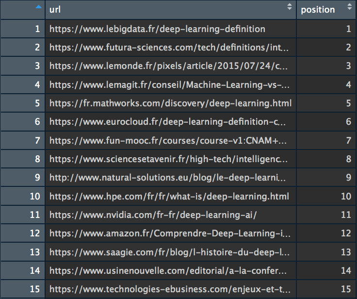
We now have a dataset (my_url_dataset) that contains the first 100 URLs that rank on the “deep learning” querie, on Google.

NB: If for any reason you want to avoid scrapping the results page of your favorite search engine yourself, note that SEMrush also offers a SERP URL retrieval function. I have added this feature into SEMrushR, the R package I created to use the SEMrush API to use the SEMrush API.

Let’s move on to recovering the Majestic data for each of these URLs.

3. Retrieve netlinking data with majesticR (API)

You may have seen it on my Twitter account, I started working on majesticR, an R package to easily connect to the Majestic API and retrieve data. It is now an official R package published on CRAN R, the reference site for R users.

For the rest of the tutorial, I used the majestic_all() function of my majesticR package which allows to retrieve, for a particular URL, the Majestic data of the URL and root domain (CF, TF, External backlinks, etc….). In order to automatically recover data from all the URLs in the list we created above with our scraper (my_url_dataset), I have integrated the majestic_all() function into a loop.

Run the following script by replacing the XXX with your Majestic API key, and enjoy life, you just created a robot that recovers the data for you:

#Get Majestic URL and Root Domain data for Google Top 100
api_Key <- "XXXXXXXXXXXXXXXXXXXXXXXXXXX"
majestic_out <- data.frame(matrix(nrow=0, ncol=142))

for (i in 1:nrow(my_url_dataset)) {
  majestic_doing <- majestic_all(my_url_dataset[i, "url"], api_Key)
  majestic_out <- rbind(majestic_out, majestic_doing)
}

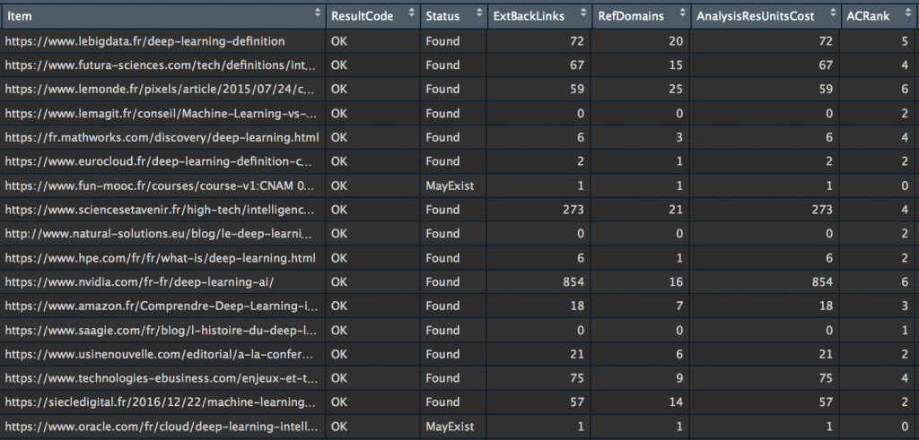
Congratulations! You have just retrieved all the netlinking data from the top 100 Google on the “deep learning” querie and everything has been stored in a dataset called “majestic_out”. We’ll be able to analyze all this!

4. Prepare the data

Before proceeding to the analysis of the correlations between the position and the netlinking variables that we have recovered, a quick data preparation step is required. We will add 3 new columns (which we will use in the rest of this tutorial), then create a new dataset that will contain only the columns we will analyze.

#Create the position variable
majestic_out <- merge(majestic_out, my_url_dataset, 
                    by.x=c("Item"),
                    by.y=c("url")) #NEW

colnames(majestic_out)[143] <- "position"
majestic_out <- majestic_out[order(majestic_out$position),]

#Keep only some variables
myvars <- c("position","ExtBackLinks","RefDomains","RefIPs", 
            "CitationFlow","TrustFlow",
            "DOMAIN_ExtBackLinks","DOMAIN_RefDomains","DOMAIN_RefIPs",
            "DOMAIN_CitationFlow","DOMAIN_TrustFlow")
subset_majestic_out <- majestic_out[myvars]

#Create 3 new columns to help us find correlations
#majestic_out$isTop3 <- 1 
#majestic_out$isTop3[majestic_out$position>3] <- 0

#majestic_out$isTop5 <- 1 
#majestic_out$isTop5[majestic_out$position>5] <- 0

#majestic_out$isTop10 <- 1 
#majestic_out$isTop10[majestic_out$position>10] <- 0

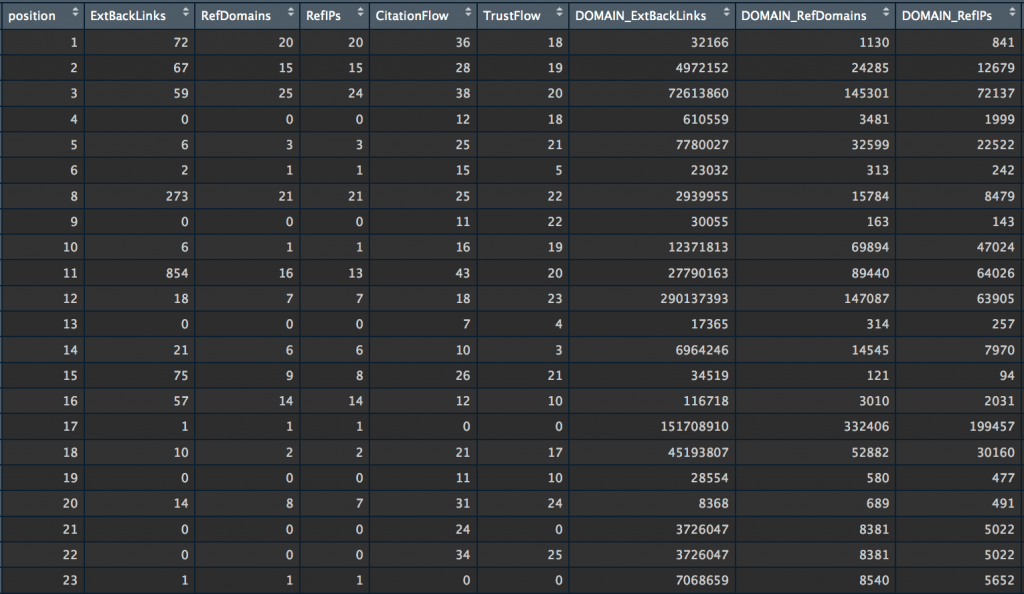
What you just did is super cool!

Data recovery and preparation are essential steps (often loved by data scientists) in any data science project. The next step is the exploratory analysis to find interesting things…

5. Analyze the correlations between netlinking and position

Let’s start with simple correlation tests between 2 variables by testing Pearson and Spearman correlations:

#Correlation between 2 continous variables
cor(subset_majestic_out$position,subset_majestic_out$ExtBackLinks, method="pearson", use = "complete.obs")
#[1] 0.02334821

cor(subset_majestic_out$position,subset_majestic_out$ExtBackLinks, method="spearman", use = "complete.obs")
#[1] -0.3977484

cor(subset_majestic_out$position,subset_majestic_out$RefDomains, method="pearson", use = "complete.obs")
#[1] -0.3045941

cor(subset_majestic_out$position,subset_majestic_out$RefDomains, method="spearman", use = "complete.obs")
#[1] -0.3963901

Here is an image to help with interpretation of these values:

If you want to evaluate the dependence between several variables at the same time, I advise you to create a correlation matrix that contains the correlation coefficients (they are used to measure the strength of the relationship between 2 variables), as well as a matrix with the p-value.

The p-value is used to measure the “quality” of correlations. It answers the following question: if there is really no correlation between X and Y, what is the probability that the random sample will produce a correlation coefficient as far away from zero (or more) as that observed in this experiment?

Let’s go back to our matrices….

my_big_matrix <- rcorr(as.matrix(subset_majestic_out))
my_big_matrix

# Extract the correlation coefficients
correlation_matrix <- round(my_big_matrix$r,2)

# Extract p-values
pvalue_matrix <- round(my_big_matrix$P,2)

Let’s finish with some visualization.

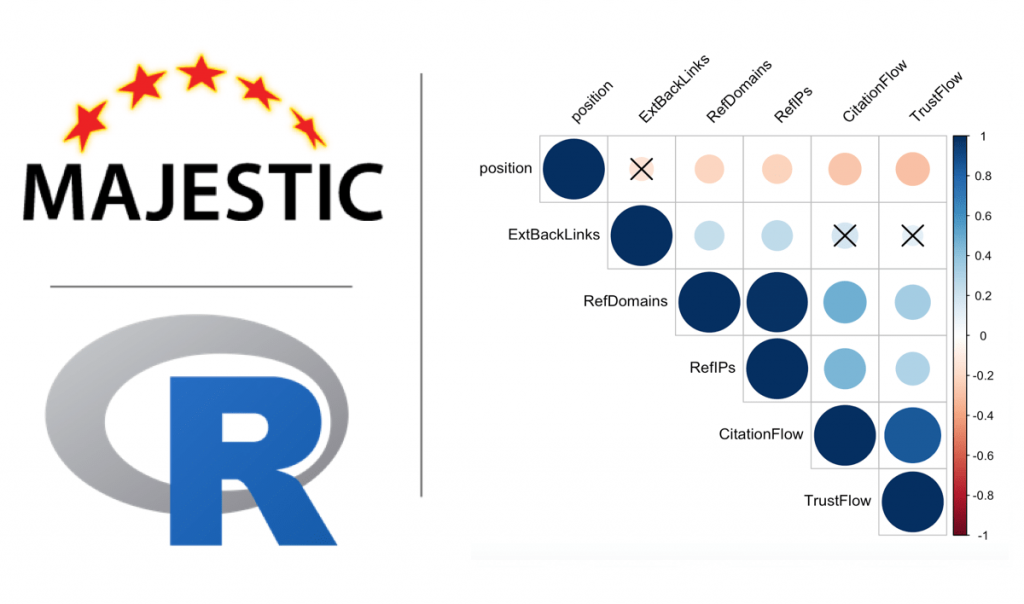
We’ll create a correlogram, a visualization of the correlation matrix. At a glance the correlogram allows to see the intensity of the correlation (the size of the circles) and their direction: the positive correlations are in blue and the negative ones in red. Crosses represent correlations that are not significant according to their p-value. I myself specified the level of significance at 0.05 (sig.level = 0.05).

corrplot(correlation_matrix, type="upper", 
         p.mat = pvalue_matrix, sig.level = 0.05, insig = "pch",
         tl.col = "black", tl.srt = 45)

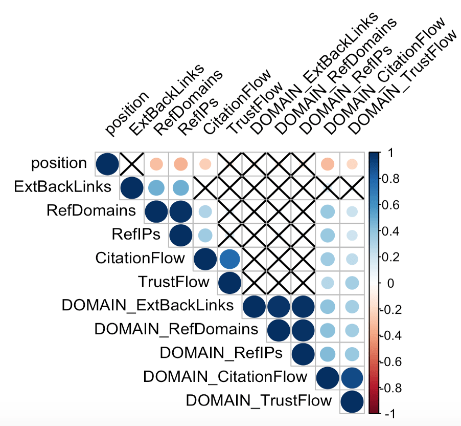
Finally, the view that brings everything together.

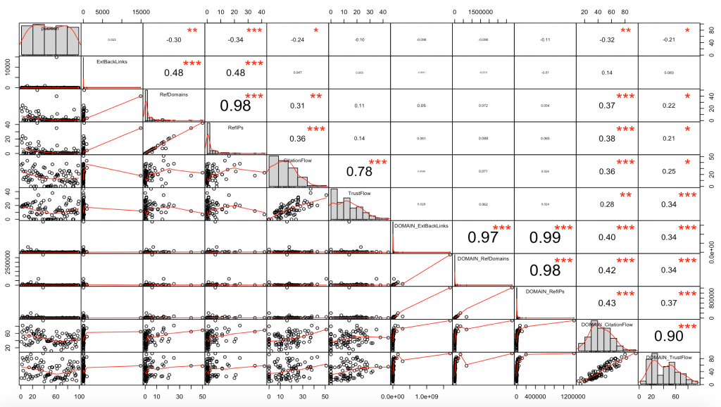
chart.Correlation(subset_majestic_out, histogram=TRUE, pch=19)

This view can be scary at first, but it all becomes clear when you know where to look!

We can see:

• The value of the correlation coefficient in the upper “triangle”
• A scatter plot visualization in the lower “triangle”, with a line that runs through the points and gives the direction of the correlation
• The distribution of each variable in the diagonal (cells with the names of the variables)
• The level of significance (p-value) of each correlation through the symbols *** (p-value very close to 0), ** (0.001), * (0.05), . (0.1) and empty space (1)

6. Interpretation of Results

The correlation coefficients between the page positions and the 10 netlinking variables seen by Majestic (ExtBacklinks, RefDomains, RefIPs, CitationFlow, TrustFlow, for URL and root domain) are quite low here.

The hypothesis that emerges from this first analysis is, however, that RefDomains, RefIPs and DOMAIN_CitationFlow seem to have some influence on the position for the “deep learning” query on Google FR.

This is a first approach to try to take advantage of the data at our disposal. It is now necessary to go further to deepen the analysis:

• Use categorical variables (Top3, Top5 and Top10) to analyze correlations
• Add other variables corresponding to the different positioning criteria (loading time, number of internal links, content size, semantic score, etc. etc…)
• Work with more observations (data increase)
• Perform a multivariate analysis using a machine learning approach in order to be as close as possible to the search engine’s behavior. The interest will be to take into account the interactions between the different variables. In other words, while the TrustFlow variable seems to have little influence on the position here, it would be wrong to conclude that it is useless for making predictions because correlations between the TrustFlow, page loading speed and position could make the TrustFlow useful. It is this type of complex and non-intuitive correlation that a machine learning model is capable of learning.

I hope you enjoyed this new tutorial! Feel free to comment if you are interested in the rest of the analysis!

To receive more R scripts : follow me on Twitter.

Follow @Remibacha